Predicting Bike Sharing Patterns

Why We’re Here

In this project, we’ll build our first neural network and use it to predict daily bike rental ridership. We start by importing all the necessary libraries.

%matplotlib inline
%load_ext autoreload
%autoreload 2
%config InlineBackend.figure_format = 'retina'

import numpy as np
import pandas as pd
import matplotlib.pyplot as plt

Loading and preparing the data

A critical step in working with neural networks is preparing the data correctly. Variables on different scales make it difficult for the network to efficiently learn the correct weights. Below, we’ve written the code to load and prepare the data.

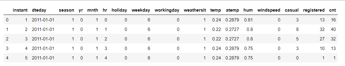
data_path = 'Bike-Sharing-Dataset/hour.csv'

rides = pd.read_csv(data_path)

rides.head()

Output:

Checking out the data

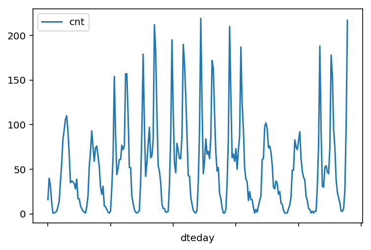
This dataset has the number of riders for each hour of each day from January 1 2011 to December 31 2012. The number of riders is split between casual and registered, summed up in the cnt column. You can see the first few rows of the data above.Below is a plot showing the number of bike riders over the first 10 days or so in the data set.

This data is pretty complicated! The weekends have lower over all ridership and there are spikes when people are biking to and from work during the week. Looking at the data above, we also have information about temperature, humidity, and windspeed, all of these likely affecting the number of riders. We’ll be trying to capture all this with our model.

rides[:24*10].plot(x='dteday', y='cnt')

Output:

Dummy variables for categorical features

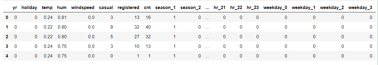
Here we have some categorical variables like season, weather, month. To include these in our model, we’ll need to make binary dummy variables. This is simple to do with Pandas thanks to get_dummies().

dummy_fields = ['season', 'weathersit', 'mnth', 'hr', 'weekday']

for each in dummy_fields:
   dummies = pd.get_dummies(rides[each], prefix=each, drop_first=False)
   rides = pd.concat([rides, dummies], axis=1)

fields_to_drop = ['instant', 'dteday', 'season', 'weathersit', 
                 'weekday', 'atemp', 'mnth', 'workingday', 'hr']

data = rides.drop(fields_to_drop, axis=1)
data.head()

Output:

Scaling target variables

To make training the network easier, we’ll standardize each of the continuous variables. That is, we’ll shift and scale the variables such that they have zero mean and a standard deviation of 1.

The scaling factors are saved so we can go backwards when we use the network for predictions.

quant_features = ['casual', 'registered', 'cnt', 'temp', 'hum', 'windspeed']

# Store scalings in a dictionary so we can convert back later
scaled_features = {}

for each in quant_features:
   mean, std = data[each].mean(), data[each].std()
   scaled_features[each] = [mean, std]
   data.loc[:, each] = (data[each] - mean)/std

Splitting the data

We’ll save the data for the last approximately 21 days to use as a test set after we’ve trained the network. We’ll use this set to make predictions and compare them with the actual number of riders.

# Save data for approximately the last 21 days 
test_data = data[-21*24:]

# Now remove the test data from the data set 
data = data[:-21*24]

# Separate the data into features and targets
target_fields = ['cnt', 'casual', 'registered']

features, targets = data.drop(target_fields, axis=1), data[target_fields]

test_features, test_targets = test_data.drop(target_fields, axis=1), test_data[target_fields]

We’ll split the data into two sets, one for training and one for validating as the network is being trained. Since this is time series data, we’ll train on historical data, then try to predict on future data (the validation set).

# Hold out the last 60 days or so of the remaining data as a validation set
train_features, train_targets = features[:-60*24], targets[:-60*24]

val_features, val_targets = features[-60*24:], targets[-60*24:]

Time to build the network

We’ve already built out the structure, now we implement both the forward pass and backwards pass through the network and also set the hyperparameters: the learning rate, the number of hidden units, and the number of training passes.

The network has two layers, a hidden layer and an output layer. The hidden layer will use the sigmoid function for activations. The output layer has only one node and is used for the regression, the output of the node is the same as the input of the node. That is, the activation function.

A function that takes the input signal and generates an output signal, but takes into account the threshold, is called an activation function. We work through each layer of our network calculating the outputs for each neuron. All of the outputs from one layer become inputs to the neurons on the next layer. This process is called forward propagation.

We use the weights to propagate signals forward from the input to the output layers in a neural network. We use the weights to also propagate error backwards from the output back into the network to update our weights. This is called backpropagation.

# importing network and defining mean squared error

from network import NeuralNetwork

def MSE(y, Y):
   return np.mean((y-Y)**2)

Unit tests

We’ll run the below unit tests to check the correctness of our network implementation. This will help us ensure if the network was implemented correctly before trying to train it.

import unittest

inputs = np.array([[0.5, -0.2, 0.1]])

targets = np.array([[0.4]])

test_w_i_h = np.array([[0.1, -0.2],
                      [0.4, 0.5],
                      [-0.3, 0.2]])

test_w_h_o = np.array([[0.3],
                      [-0.1]])

class TestMethods(unittest.TestCase):
   
   ##########
   # Unit tests for data loading
   ##########
   
   def test_data_path(self):
       # Test that file path to dataset has been unaltered
      self.assertTrue(data_path.lower() == 'bike-sharing-dataset/hour.csv')
      
  def test_data_loaded(self):
      # Test that data frame loaded
      self.assertTrue(isinstance(rides, pd.DataFrame))
  
  ##########
  # Unit tests for network functionality
  ##########
  def test_activation(self):
      network = NeuralNetwork(3, 2, 1, 0.5)
      # Test that the activation function is a sigmoid
      self.assertTrue(np.all(network.activation_function(0.5) == 1/(1+np.exp(-0.5))))

  def test_train(self):
      # Test that weights are updated correctly on training
      network = NeuralNetwork(3, 2, 1, 0.5)
       network.weights_input_to_hidden = test_w_i_h.copy()
       network.weights_hidden_to_output = test_w_h_o.copy()
       
       network.train(inputs, targets)
       self.assertTrue(np.allclose(network.weights_hidden_to_output, 
                                   np.array([[ 0.37275328], 
                                             [-0.03172939]])))
       self.assertTrue(np.allclose(network.weights_input_to_hidden,
                                   np.array([[ 0.10562014, -0.20185996], 
                                             [0.39775194, 0.50074398], 
                                             [-0.29887597, 0.19962801]])))

   def test_run(self):
       # Test correctness of run method
       network = NeuralNetwork(3, 2, 1, 0.5)
       network.weights_input_to_hidden = test_w_i_h.copy()
       network.weights_hidden_to_output = test_w_h_o.copy()
       self.assertTrue(np.allclose(network.run(inputs), 0.09998924))>

suite = unittest.TestLoader().loadTestsFromModule(TestMethods())

unittest.TextTestRunner().run(suite)

Output:
    ----------------------------------------------------------------------
    Ran 5 tests in 0.012s    
    OK
    <unittest.runner.TextTestResult run=5 errors=0 failures=0>

Training the network

The strategy here is to find hyperparameters such that the error on the training set is low, but we’re not overfitting to the data. If we train the network too long or have too many hidden nodes, it can become overly specific to the training set and will fail to generalize to the validation set. That is, the loss on the validation set will start increasing as the training set loss drops.

We’ll also be using a method know as Stochastic Gradient Descent (SGD) to train the network. The idea is that for each training pass, we grab a random sample of the data instead of using the whole data set. We use many more training passes than with normal gradient descent, but each pass is much faster. This ends up training the network more efficiently.

Choose the number of iterations

This is the number of batches of samples from the training data we’ll use to train the network. The more iterations, the better the model will fit the data. However, this process can have sharply diminishing returns and can waste computational resources if we use too many iterations.

We want to find a number here where the network has a low training loss, and the validation loss is at a minimum. The ideal number of iterations would be a level that stops shortly after the validation loss is no longer decreasing.

Choose the learning rate

This scales the size of weight updates. If this is too big, the weights tend to explode and the network fails to fit the data. Normally a good choice to start at is 0.1; however, if we effectively divide the learning rate by n_records, try starting out with a learning rate of 1.

In either case, if the network has problems fitting the data, try reducing the learning rate. Note that the lower the learning rate, the smaller the steps are in the weight updates and the longer it takes for the neural network to converge.

Choose the number of hidden nodes

In a model where all the weights are optimized, the more hidden nodes, the more accurate the predictions of the model will be. (A fully optimized model could have weights of zero, after all.) However, the more hidden nodes you have, the harder it will be to optimize the weights of the model, and the more likely it will be that suboptimal weights will lead to overfitting. With overfitting, the model will memorize the training data instead of learning the true pattern, and won’t generalize well to unseen data.

Try a few different numbers and see how it affects the performance. We can look at the losses dictionary for a metric of the network performance. If the number of hidden units is too low, then the model won’t have enough space to learn and if it is too high there are too many options for the direction that the learning can take.

The trick here is to find the right balance in number of hidden units you choose. We’ll generally find that the best number of hidden nodes to use ends up being between the number of input and output nodes.

import sys

from network import iterations, learning_rate, hidden_nodes, output_nodes

N_i = train_features.shape[1]
network = NeuralNetwork(N_i, hidden_nodes, output_nodes, learning_rate)

losses = {'train':[], 'validation':[]}
for ii in range(iterations):
   # Go through a random batch of 128 records from the training data set
   batch = np.random.choice(train_features.index, size=128)
   X, y = train_features.ix[batch].values, train_targets.ix[batch]['cnt']
                            
   network.train(X, y)
   
   # Printing out the training progress
   train_loss = MSE(network.run(train_features).T, train_targets['cnt'].values)
   val_loss = MSE(network.run(val_features).T, val_targets['cnt'].values)
   sys.stdout.write("\rProgress: {:2.1f}".format(100 * ii/float(iterations)) \
                    + "% ... Training loss: " + str(train_loss)[:5] \
                   + " ... Validation loss: " + str(val_loss)[:5])
   sys.stdout.flush()
   
   losses['train'].append(train_loss)
   losses['validation'].append(val_loss)

Output:
Progress: 0.1% ... Training loss: 71.64 ... Validation loss: 18.54
...
...
Progress: 100.0% ... Training loss: 0.076 ... Validation loss: 0.160

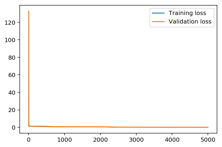
Plotting the train and validation loss

plt.plot(losses['train'], label='Training loss')
plt.plot(losses['validation'], label='Validation loss')
plt.legend()
_ = plt.ylim()

Output:

Check out your predictions

Here, we use the test data to view how well your network is modeling the data.

fig, ax = plt.subplots(figsize=(8,4))

mean, std = scaled_features['cnt']
predictions = network.run(test_features).T*std + mean
ax.plot(predictions[0], label='Prediction')
ax.plot((test_targets['cnt']*std + mean).values, label='Data')
ax.set_xlim(right=len(predictions))
ax.legend()

dates = pd.to_datetime(rides.ix[test_data.index]['dteday'])
dates = dates.apply(lambda d: d.strftime('%b %d'))
ax.set_xticks(np.arange(len(dates))[12::24])
_ = ax.set_xticklabels(dates[12::24], rotation=45)

Output:

Observations:

The demand seems high in the mid-week of December and the model seems to correctly predict the trend before christmas since model did not receive any information about the change in trend due to a holiday week,the model could not precisely predict the data during christmas.

Conclusion

We successfully built a numpy based neural network for predicting the daily bike rentals by transforming and scaling the data according to the input requirement of our neural network. The model does a decent job on most days except the holiday season which might be due to lack of information on holidays.