Face Generation with GAN
Why We’re Here
In this project, we’ll define and train a DCGAN on a dataset of faces. Our goal is to get a generator network to generate new images of faces that look as realistic as possible!
The project will be broken down into a series of tasks from loading in data to defining and training adversarial networks. At the end of the notebook, we’ll be able to visualize the results of our trained Generator to see how it performs; our generated samples should look like fairly realistic faces with small amounts of noise.
Get the Data
We’ll be using the CelebFaces Attributes Dataset (CelebA) to train our adversarial networks.
This dataset is more complex than the number datasets (like MNIST or SVHN) we’ve been working with, and so, we should prepare to define deeper networks and train them for a longer time to get good results. It’s better if we utilize a GPU for training.
Pre-processed Data
Since the project’s main focus is on building the GANs, we’ve done some of the pre-processing before. Each of the CelebA images has been cropped to remove parts of the image that don’t include a face, then resized down to 64x64x3 NumPy images. Some sample data is show below.
If you are working locally, you can download this data by clicking here
This is a zip file that we’ll need to extract in the home directory of this notebook for further loading and processing. After extracting the data, we should be left with a directory of data processed_celeba_small/
# can comment out after executing
# !unzip processed_celeba_small.zip

data_dir = 'processed_celeba_small/'

import pickle as pkl
import matplotlib.pyplot as plt
import numpy as np
import problem_unittests as tests
#import helper

%matplotlib inline
Visualize the CelebA Data
The CelebA dataset contains over 200,000 celebrity images with annotations. Since we’re going to be generating faces, we won’t need the annotations, we’ll only need the images. Note that these are color images with 3 color channels (RGB) each.
Pre-process and Load the Data
Since the project’s main focus is on building the GANs, we’ve done some of the pre-processing for you. Each of the CelebA images has been cropped to remove parts of the image that don’t include a face, then resized down to 64x64x3 NumPy images. This pre-processed dataset is a smaller subset of the very large CelebA data.
There are a few other steps that we’ll need to transform this data and create a DataLoader.
Creating get_dataloader function, such that it satisfies these requirements:
- a. Our images should be square, Tensor images of size
image_size x image_sizein the x and y dimension. - b. Our function should return a DataLoader that shuffles and batches these Tensor images.
ImageFolder
To create a dataset given a directory of images, it’s recommended to use PyTorch’s ImageFolder wrapper, with a root directory processed_celeba_small/ and data transformation passed in.
# necessary imports
import torch
from torchvision import datasets
from torchvision import transforms

def get_dataloader(batch_size, image_size, data_dir='processed_celeba_small/'):
   """
   Batch the neural network data using DataLoader
   :param batch_size: The size of each batch; the number of images in a batch
   :param img_size: The square size of the image data (x, y)
   :param data_dir: Directory where image data is located
   :return: DataLoader with batched data
   """

   # Implement function and return a dataloader
   # resize and normalize the images
   transform = transforms.Compose([transforms.Resize(image_size),
                                   transforms.ToTensor()])

   # define datasets using ImageFolder
   train_dataset = datasets.ImageFolder(data_dir, transform)

   # create and return DataLoaders
   data_loader = torch.utils.data.DataLoader(dataset=train_dataset, batch_size=batch_size, shuffle=True)

   return data_loader
Create a DataLoader
Creating a DataLoader celeba_train_loader with appropriate hyperparameters. Call the above function and create a dataloader to view images.
- a. You can decide on any reasonable
batch_sizeparameter - b. Your
image_sizemust be32. Resizing the data to a smaller size will make for faster training, while still creating convincing images of faces!
# Define function hyperparameters
batch_size = 32

img_size = 32

# Call your function and get a dataloader
celeba_train_loader = get_dataloader(batch_size, img_size)
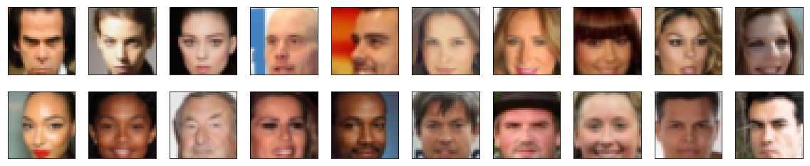
Next, we can view some images!
Note: We’ll need to convert the Tensor images into a NumPy type and transpose the dimensions to correctly display an image, suggested imshow code is below, but it may not be perfect.
# helper display function
def imshow(img):
   npimg = img.numpy()
   plt.imshow(np.transpose(npimg, (1, 2, 0)))

# obtain one batch of training images
dataiter = iter(celeba_train_loader)
images, _ = dataiter.next() # _ for no labels

# plot the images in the batch, along with the corresponding labels
fig = plt.figure(figsize=(20, 4))
plot_size=20
for idx in np.arange(plot_size):
   ax = fig.add_subplot(2, plot_size/2, idx+1, xticks=[], yticks=[])
   imshow(images[idx])
Output:
Pre-process the image data and scale it to a pixel range of -1 to 1
We need to do a bit of pre-processing; we know that the output of a tanh activated generator will contain pixel values in a range from -1 to 1, and so, we need to rescale our training images to a range of -1 to 1. (Right now, they are in a range from 0-1.)
# Complete the scale function
def scale(x, feature_range=(-1, 1)):
   ''' Scale takes in an image x and returns that image, scaled
      with a feature_range of pixel values from -1 to 1.
      This function assumes that the input x is already scaled from 0-1.'''
   # assume x is scaled to (0, 1)
   # scale to feature_range and return scaled x
   min,max = feature_range
   x = x*(max - min) + min
   return x

# check scaled range
# should be close to -1 to 1
img = images[0]
scaled_img = scale(img)

print('Min: ', scaled_img.min())
print('Max: ', scaled_img.max())
Output:
    Min:  tensor(-0.9922)
    Max:  tensor(1.)
Define the Model
A GAN is comprised of two adversarial networks, a discriminator and a generator.
Discriminator
Our first task will be to define the discriminator. This is a convolutional classifier like you’ve built before, only without any maxpooling layers. To deal with this complex data, it’s suggested we use a deep network with normalization.
Creating the Discriminator class such that it satisfies these requirements:
- a. The inputs to the discriminator are 32x32x3 tensor images
- b. The output should be a single value that will indicate whether a given image is real or fake
import torch.nn as nn
import torch.nn.functional as F
# helper to build a convolution layer def conv(in_channels,out_channels,kernel_size,stride = 2,padding = 1,batch_norm = True): layers = [] conv_layer = nn.Conv2d(in_channels = in_channels,out_channels = out_channels, kernel_size = kernel_size,stride = stride,padding = padding,bias= False) layers.append(conv_layer) if batch_norm == True: layers.append(nn.BatchNorm2d(out_channels)) return nn.Sequential(*layers) class Discriminator(nn.Module): def __init__(self, conv_dim=32): """ Initialize the Discriminator Module :param conv_dim: The depth of the first convolutional layer """ super(Discriminator, self).__init__() self.conv_dim = conv_dim # covolution layers # input 32 x 32 x 3 -> output 16 x 16 x 32 self.conv1 = conv(3,conv_dim,4,batch_norm = False) # input 16 x 16 x 32 -> output 8 x 8 x 64 self.conv2 = conv(conv_dim,conv_dim*2,4) # input 8 x 8 x 64 -> output 4 x 4 x 128 self.conv3 = conv(conv_dim*2,conv_dim*4,4) # input 4 x 4 x 128 -> output 2 x 2 x 256 self.conv4 = conv(conv_dim*4,conv_dim*8,4) # classification layers self.fc = nn.Linear(conv_dim*8*2*2,1) def forward(self, x): """ Forward propagation of the neural network :param x: The input to the neural network :return: Discriminator logits; the output of the neural network """ # define feedforward behavior x = F.leaky_relu(self.conv1(x),0.2) x = F.leaky_relu(self.conv2(x),0.2) x = F.leaky_relu(self.conv3(x),0.2) x = F.leaky_relu(self.conv4(x),0.2) # output x = x.view(-1,self.conv_dim*8*2*2) x = self.fc(x) return x tests.test_discriminator(Discriminator)
Output:
    Tests Passed
Generator
The generator should upsample an input and generate a new image of the same size as our training data 32x32x3. This should be mostly transpose convolutional layers with normalization applied to the outputs.
Creating the Generator class such that it satisfies these requirements:
- a. The inputs to the generator are vectors of some length
z_size - b. The output should be a image of shape
32x32x3
def deconv(in_channels, out_channels, kernel_size, stride=2, padding=1, batch_norm=True):
   # create a sequence of transpose + optional batch norm layers
   layers = []
   transpose_conv_layer = nn.ConvTranspose2d(in_channels, out_channels,
                                             kernel_size, stride, padding, bias=False)
   # append transpose convolutional layer
   layers.append(transpose_conv_layer)

   if batch_norm:
       # append batchnorm layer
       layers.append(nn.BatchNorm2d(out_channels))

   return nn.Sequential(*layers)

class Generator(nn.Module):

   def __init__(self, z_size, conv_dim = 32):
       """
       Initialize the Generator Module
       :param z_size: The length of the input latent vector, z
       :param conv_dim: The depth of the inputs to the *last* transpose convolutional layer
       """
       super(Generator, self).__init__()

       self.conv_dim = conv_dim

       self.fc = nn.Linear(z_size,conv_dim*8*2*2)

       self.t_conv1 = deconv(conv_dim*8,conv_dim*4,4)
       self.t_conv2 = deconv(conv_dim*4,conv_dim*2,4)
       self.t_conv3 = deconv(conv_dim*2,conv_dim,4)
       self.t_conv4 = deconv(conv_dim,3,4,batch_norm = False)

   def forward(self, x):
       """
       Forward propagation of the neural network
       :param x: The input to the neural network
       :return: A 32x32x3 Tensor image as output
       """
       # define feedforward behavior
       x = self.fc(x)
       x = x.view(-1,self.conv_dim*8,2,2)

       x = F.relu(self.t_conv1(x))
       x = F.relu(self.t_conv2(x))
       x = F.relu(self.t_conv3(x))
       x = F.tanh(self.t_conv4(x))

       return x

tests.test_generator(Generator)
Output:
    Tests Passed
Initialize the weights of your networks
To help your models converge, you should initialize the weights of the convolutional and linear layers in your model. From reading the original DCGAN paper, they say:
All weights were initialized from a zero-centered Normal distribution with standard deviation 0.02.
So, our next task will be to define a weight initialization function that does just this!
Creating the weight initialization function such that:
- a. It should initialize only convolutional and linear layers
- b. Initialize the weights to a normal distribution, centered around 0, with a standard deviation of 0.02.
- c. The bias terms, if they exist, may be left alone or set to 0.
def weights_init_normal(m):
   """
   Applies initial weights to certain layers in a model .
   The weights are taken from a normal distribution
   with mean = 0, std dev = 0.02.
   :param m: A module or layer in a network
   """
   # classname will be something like:
   # `Conv`, `BatchNorm2d`, `Linear`, etc.
   classname = m.__class__.__name__

   # Apply initial weights to convolutional and linear layers
   if classname.find('Conv') != -1 or classname.find('Linear') != -1:
       nn.init.normal_(m.weight.data, 0, 0.02)
   if hasattr(m, 'bias') and m.bias is not None:
       m.bias.data.fill_(0)
Build complete network
Defining the models’ hyperparameters and instantiate the discriminator and generator from the classes defined above.
def build_network(d_conv_dim, g_conv_dim, z_size):
   # define discriminator and generator
   D = Discriminator(d_conv_dim)
   G = Generator(z_size=z_size, conv_dim=g_conv_dim)

   # initialize model weights
   D.apply(weights_init_normal)
   G.apply(weights_init_normal)

   print(D)
   print()
   print(G)

   return D, G
Define model hyperparameters
# Define model hyperparams
d_conv_dim = 32
g_conv_dim = 32
z_size = 100

D, G = build_network(d_conv_dim, g_conv_dim, z_size)
Output:
    Discriminator(
      (conv1): Sequential(
        (0): Conv2d(3, 32, kernel_size=(4, 4), stride=(2, 2), padding=(1, 1), bias=False)
      )
      (conv2): Sequential(
        (0): Conv2d(32, 64, kernel_size=(4, 4), stride=(2, 2), padding=(1, 1), bias=False)
        (1): BatchNorm2d(64, eps=1e-05, momentum=0.1, affine=True, track_running_stats=True)
      )
      (conv3): Sequential(
        (0): Conv2d(64, 128, kernel_size=(4, 4), stride=(2, 2), padding=(1, 1), bias=False)
        (1): BatchNorm2d(128, eps=1e-05, momentum=0.1, affine=True, track_running_stats=True)
      )
      (conv4): Sequential(
        (0): Conv2d(128, 256, kernel_size=(4, 4), stride=(2, 2), padding=(1, 1), bias=False)
        (1): BatchNorm2d(256, eps=1e-05, momentum=0.1, affine=True, track_running_stats=True)
      )
      (fc): Linear(in_features=1024, out_features=1, bias=True)
    )

    Generator(
      (fc): Linear(in_features=100, out_features=1024, bias=True)
      (t_conv1): Sequential(
        (0): ConvTranspose2d(256, 128, kernel_size=(4, 4), stride=(2, 2), padding=(1, 1), bias=False)
        (1): BatchNorm2d(128, eps=1e-05, momentum=0.1, affine=True, track_running_stats=True)
      )
      (t_conv2): Sequential(
        (0): ConvTranspose2d(128, 64, kernel_size=(4, 4), stride=(2, 2), padding=(1, 1), bias=False)
        (1): BatchNorm2d(64, eps=1e-05, momentum=0.1, affine=True, track_running_stats=True)
      )
      (t_conv3): Sequential(
        (0): ConvTranspose2d(64, 32, kernel_size=(4, 4), stride=(2, 2), padding=(1, 1), bias=False)
        (1): BatchNorm2d(32, eps=1e-05, momentum=0.1, affine=True, track_running_stats=True)
      )
      (t_conv4): Sequential(
        (0): ConvTranspose2d(32, 3, kernel_size=(4, 4), stride=(2, 2), padding=(1, 1), bias=False)
      )
    )
Training on GPU
Checking if we can train on GPU. Here, we’ll set this as a boolean variable train_on_gpu. Later, we’ll be responsible for making sure that
- a. Models,
- b. Model inputs, and
- c. Loss function arguments
Are moved to GPU, where appropriate.
import torch

# Check for a GPU
train_on_gpu = torch.cuda.is_available()
if not train_on_gpu:
   print('No GPU found. Please use a GPU to train your neural network.')
else:
   print('Training on GPU!')
Output:
    Training on GPU!
Discriminator and Generator Losses
Now we need to calculate the losses for both types of adversarial networks.
Discriminator Losses
- a. For the discriminator, the total loss is the sum of the losses for real and fake images,
d_loss = d_real_loss + d_fake_loss. - b. Remember that we want the discriminator to output 1 for real images and 0 for fake images, so we need to set up the losses to reflect that.
Generator Loss
The generator loss will look similar only with flipped labels. The generator’s goal is to get the discriminator to think its generated images are real.
Complete real and fake loss functions
We can use either cross entropy or a least squares error loss to complete the following real_loss and fake_loss functions.
def real_loss(D_out,smooth=False):
   batch_size = D_out.size(0)
   if smooth:
       # smooth, real labels = 0.9
       labels = torch.ones(batch_size)*0.9
   else:
       labels = torch.ones(batch_size) # real labels = 1
   # move labels to GPU if available
   if train_on_gpu:
       labels = labels.cuda()
   # binary cross entropy with logits loss
   criterion = nn.BCEWithLogitsLoss()
   # calculate loss
   loss = criterion(D_out.squeeze(), labels)
   return loss

def fake_loss(D_out):
   '''Calculates how close discriminator outputs are to being fake.
      param, D_out: discriminator logits
      return: fake loss'''
   batch_size = D_out.size(0)
   labels = torch.zeros(batch_size) # fake labels = 0
   if train_on_gpu:
       labels = labels.cuda()
   criterion = nn.BCEWithLogitsLoss()
   # calculate loss
   loss = criterion(D_out.squeeze(), labels)
   return loss
Optimizers
Define optimizers for your Discriminator (D) and Generator (G)
Define optimizers for your models with appropriate hyperparameters.
import torch.optim as optim

# Create optimizers for the discriminator D and generator G
lr = 0.0002
beta1=0.5
beta2=0.999 # default value

# Create optimizers for the discriminator and generator
d_optimizer = optim.Adam(D.parameters(), lr, [beta1, beta2])
g_optimizer = optim.Adam(G.parameters(), lr, [beta1, beta2])
Training
Training will involve alternating between training the discriminator and the generator. We’ll use your functions real_loss and fake_loss to help you calculate the discriminator losses.
- a. We should train the discriminator by alternating on real and fake images
- b. Then the generator, which tries to trick the discriminator and should have an opposing loss function
Saving Samples
We’ve been given some code to print out some loss statistics and save some generated “fake” samples.
Setup the training function
Keep in mind that, if you’ve moved your models to GPU, you’ll also have to move any model inputs to GPU.
def train(D, G, n_epochs, print_every=50):
   '''Trains adversarial networks for some number of epochs
      param, D: the discriminator network
      param, G: the generator network
      param, n_epochs: number of epochs to train for
      param, print_every: when to print and record the models' losses
      return: D and G losses'''

   # move models to GPU
   if train_on_gpu:
       D.cuda()
       G.cuda()

   # keep track of loss and generated, "fake" samples
   samples = []
   losses = []

   # Get some fixed data for sampling. These are images that are held
   # constant throughout training, and allow us to inspect the model's performance
   sample_size=16
   fixed_z = np.random.uniform(-1, 1, size=(sample_size, z_size))
   fixed_z = torch.from_numpy(fixed_z).float()
   # move z to GPU if available
   if train_on_gpu:
       fixed_z = fixed_z.cuda()

   # epoch training loop
   for epoch in range(n_epochs):

       # batch training loop
       for batch_i, (real_images, _) in enumerate(celeba_train_loader):

           batch_size = real_images.size(0)
           real_images = scale(real_images)

           # ============================================
           #            TRAIN THE DISCRIMINATOR
           # ============================================

           d_optimizer.zero_grad()
           # 1. Train the discriminator on real and fake images

           # Train with real images
           if train_on_gpu:
               real_images = real_images.cuda()

           D_real = D(real_images)
           d_real_loss = real_loss(D_real)

           # 2. Train with fake images

           # Generate fake images
           z = np.random.uniform(-1, 1, size=(batch_size, z_size))
           z = torch.from_numpy(z).float()
           # move x to GPU, if available
           if train_on_gpu:
               z = z.cuda()
           fake_images = G(z)

           # Compute the discriminator losses on fake images
           D_fake = D(fake_images)
           d_fake_loss = fake_loss(D_fake)

           # add up loss and perform backprop
           d_loss = d_real_loss + d_fake_loss
           d_loss.backward()
           d_optimizer.step()


           # =========================================
           #            TRAIN THE GENERATOR
           # =========================================
           g_optimizer.zero_grad()

           # 1. Train with fake images and flipped labels

           # Generate fake images
           z = np.random.uniform(-1, 1, size=(batch_size, z_size))
           z = torch.from_numpy(z).float()
           if train_on_gpu:
               z = z.cuda()
           fake_images = G(z)

           # Compute the discriminator losses on fake images
           # using flipped labels!
           D_fake = D(fake_images)
           g_loss = real_loss(D_fake) # use real loss to flip labels

           # perform backprop
           g_loss.backward()
           g_optimizer.step()


           # ===============================================
           #              END OF CODE
           # ===============================================

           # Print some loss stats
           if batch_i % print_every == 0:
               # append discriminator loss and generator loss
               losses.append((d_loss.item(), g_loss.item()))
               # print discriminator and generator loss
               print('Epoch [{:5d}/{:5d}] | d_loss: {:6.4f} | g_loss: {:6.4f}'.format(
                       epoch+1, n_epochs, d_loss.item(), g_loss.item()))


       ## AFTER EACH EPOCH##
       # this code assumes your generator is named G, feel free to change the name
       # generate and save sample, fake images
       G.eval() # for generating samples
       samples_z = G(fixed_z)
       samples.append(samples_z)
       G.train() # back to training mode

   # Save training generator samples
   with open('train_samples.pkl', 'wb') as f:
       pkl.dump(samples, f)

   # finally return losses
   return losses
Set the number of training epochs and train the GAN!
# set number of epochs
n_epochs = 10

# call training function
losses = train(D, G, n_epochs=n_epochs)
Output:
    Epoch [1/10] | d_loss: 1.4375 | g_loss: 0.8283
    ..
    ..
    Epoch [10/10] | d_loss: 0.2544 | g_loss: 3.4693
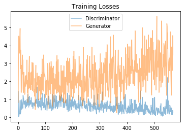
Training loss
Plot the training losses for the generator and discriminator, recorded after each epoch.
fig, ax = plt.subplots()
losses = np.array(losses)
plt.plot(losses.T[0], label='Discriminator', alpha=0.5)
plt.plot(losses.T[1], label='Generator', alpha=0.5)
plt.title("Training Losses")
plt.legend()
Output:
Generator samples from training
View samples of images from the generator, and observing the strengths and weaknesses of our trained models.
# helper function for viewing a list of passed in sample images
def view_samples(epoch, samples):
   fig, axes = plt.subplots(figsize=(16,4), nrows=2, ncols=8, sharey=True, sharex=True)
   for ax, img in zip(axes.flatten(), samples[epoch]):
       img = img.detach().cpu().numpy()
       img = np.transpose(img, (1, 2, 0))
       img = ((img + 1)*255 / (2)).astype(np.uint8)
       ax.xaxis.set_visible(False)
       ax.yaxis.set_visible(False)
       im = ax.imshow(img.reshape((32,32,3)))

# Load samples from generator, taken while training
with open('train_samples.pkl', 'rb') as f:
   samples = pkl.load(f)

_ = view_samples(-1, samples)
Output:
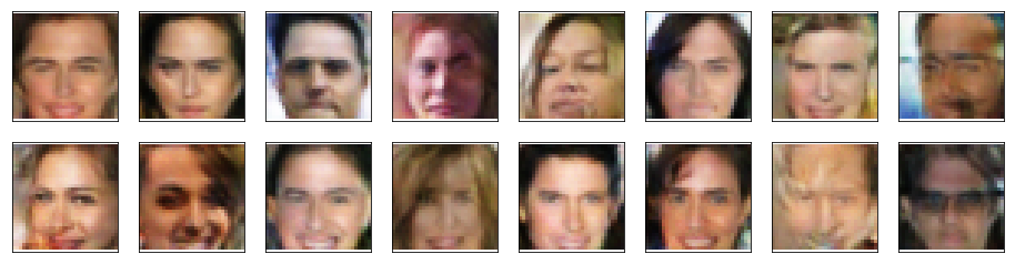
Conclusion
We’ve successfully developed a deep convolutional generative adversarial network (DCGAN) to generate realistic human faces from random noise. The model was trained on the CelebFaces Attributes Dataset (CelebA), which contains over 200,000 celebrity images. The trained model is able to generate new images of faces that look as realistic as possible.
The complete implementation can be found in the GitHub repository.